How to simulate using FEA in PTC Creo

A step-by-step tutorial for analyzing beam stress and deformation.

Finite element analysis (FEA) is one of the most critical tools in a simulation engineer’s toolbox. Understanding how a component or assembly will deform and the stresses generated during loading helps engineers design everything from phone cases to jumbo jets.

This tutorial uses revision 6.0.4.0 of Creo Parametric and Creo Simulate. A newer software version might yield different results and graphics. Like most CAD packages, Creo allows simulation engineers to design and simulate within one environment, using Creo Parametric for the modeling and Creo Simulate for the analysis. Unless you’re a top-tier simulation engineer, you probably can’t choose the analysis tools you use.

Cost, availability, computing power, customer preference and feature availability are all factors in choosing the CAD and analysis packages used in a study. Five years ago, the best CAD and simulation packages could perform both functions but had specialties. Today, CAD packages have more advanced simulation functions, and straight simulation software packages have better modeling capabilities. Beyond meeting in the middle of some design and simulation axis, most companies are improving file transfers and pulling models or studies from other programs.

In this example, we simulate beam deflection the “long way” to show the meshing process in detail. However, the problem can be simplified by defining the object as a beam element, reducing the mesh from 12 elements shown in the upcoming example to one. This is generally recommended (when possible) to keep computations down.

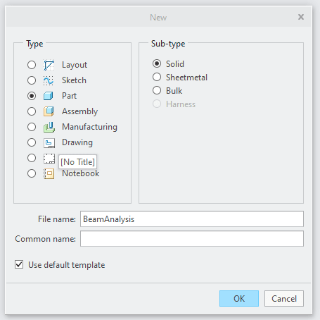
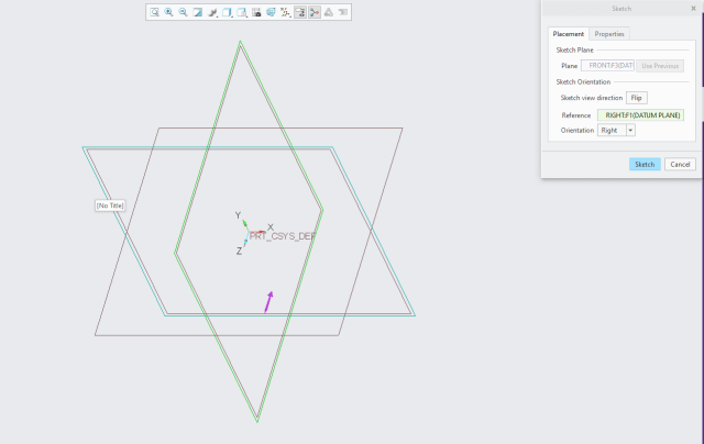
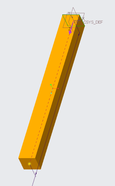
The first step in a straight beam deflection problem is creating the beam. I created a square 10 x 10-inch section and extruded it 100 inches. This is a big, beefy beam that would be embarrassingly over-engineered for most applications, especially if it’s intended to be made from steel.

The first step is to create a part for the analysis. (Image: Tom Spendlove.)

Next, create the sketch and decide which planes to use. (Image: Tom Spendlove.)

Then, create a 2D sketch and a 3D beam. (Image: Tom Spendlove.)

After we are comfortable with the CAD model generated, the next step is adding the information required to run a simulation. Generally, the pre-processing steps are adding loading, adding constraints, generating a mesh and assigning the material. Adding constraints tells the software which degrees of freedom are held in the model. The simplest way to do this is to open the “Constraints” menu and choose a surface to be constrained.

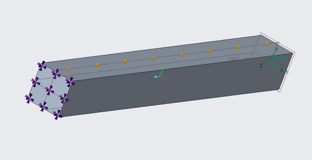
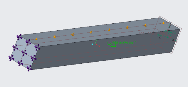
In this example of a cantilever beam-type load, we fix one end of the beam and push on the beam’s top surface with a distributed load. The green box in the “Constraint” window shows which selection is active, and in this case, it prompts us to choose the geometry that will be constrained. The software allows for constraining motion in the X, Y and Z axes and then rotation around the X, Y and Z axes. The default when you choose a surface is to constrain all six degrees of freedom.

Open the “Constraint” menu and select a surface to constrain. (Image: Tom Spendlove.)

This surface shows that it is constrained. (Image: Tom Spendlove.)

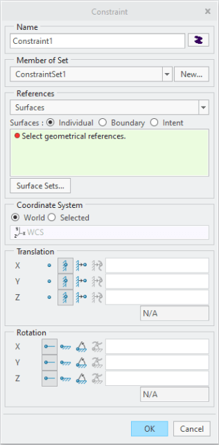
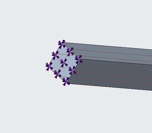
The blue arrows at the end of the part show that it is fixed in the X, Y and Z directions. If a part is designed to slide or rotate, you can build a different constraint set that shows different visuals.

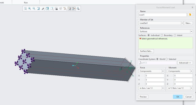
Adding forces or moments to the model is done in the same manner as adding the constraints. Theoretically, adding the mesh, loads, constraints and material can be done in any order, but all of these parameters must be in place before running the simulation. Looking again at the menu and finding the green box that indicates what needs to be selected, the user can specify where this load is applied and then specify if the load is a force or a moment, the magnitude of that load and the units.

Note that Creo will do what you tell it to do. If you want to design your components in English units and then create the load cases in metric units, Creo will rectify those two different systems. Therefore, it is important to understand exactly what you type into these different windows, and to watch the inputs and outputs closely to ensure you get the information you require from a study.

Next, add forces or moments. (Image: Tom Spendlove.)

The model now shows constraints and forces. (Image: Tom Spendlove.)

Theoretically, the only material property required to run a static FEA study like this is Poisson’s ratio. It’s unlikely that you would know the Poisson’s ratio of a material without knowing any other properties. If that ever happens, it’s possible to create a dummy material name and add that information for a study.

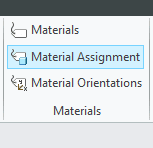
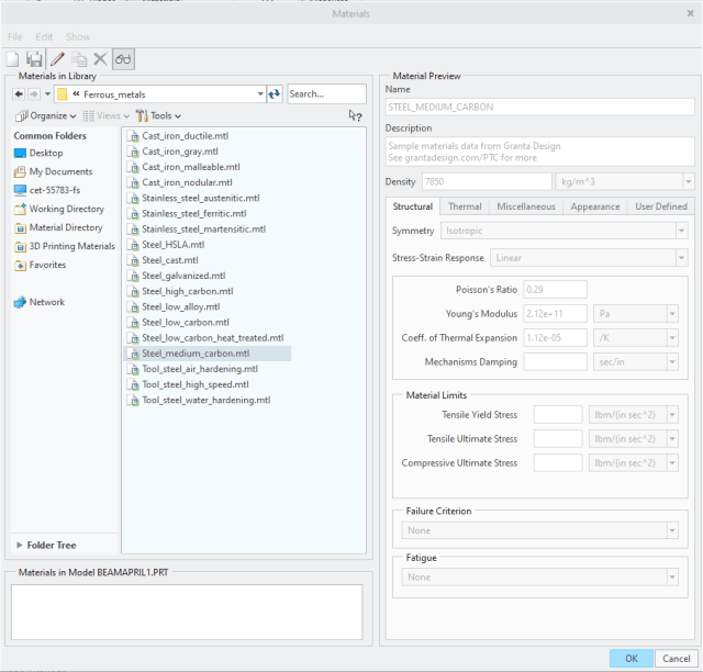
The more conventional method of assigning a material is to tell Creo what material you’re using and then pull all the material properties from the database. PTC has a partnership with Ansys to use the Granta Materials Intelligence system, and that’s the easiest way for me to assign a material to a component. If we were running a study on an assembly of parts, every component could have its own material assigned.

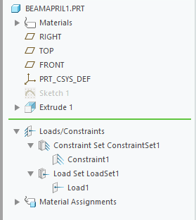
After a material is assigned in the “Structural” tab, the Poisson’s ratio, Young’s modulus and coefficient of thermal expansion (CTE) fields are populated for the generic material chosen; in this case, medium carbon steel. An engineer trying to analyze a specific grade of material might have a better handle on the exact material properties of their application. Adding those fine details would ultimately lead to better fidelity between the simulation study and reality. Two ways to mentally check off that the material is correctly assigned are the tag icon that drops next to the component in the main view window, and a materials note in the design tree for the component.

Assign a material to the model. (Image: Tom Spendlove.)

Materials and properties from PTC’s Granta directory. (Image: Tom Spendlove.)

The material tag on the model shows that a material is assigned. (Image: Tom Spendlove.)

The feature tree also shows that a material is assigned. (Image: Tom Spendlove.)

The AutoGEM mesher can build a mesh of elements and nodes for the study. Theoretically, this mesh is the only thing needed to run the finite element study. The geometry is there, but the meshing nodes and elements are used for the analysis.

The AutoGEM mesher sets up a mesh and gives mesh information. (Image: Tom Spendlove.)

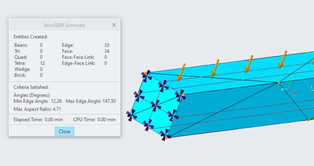
Advanced users can change how the mesh is built. The design tradeoff is that smaller elements yield better results but require more time and stronger computing power.

Start a new analysis from the “Analyses and Studies” icon. (Image: Tom Spendlove.)

Set up the parameters of the study. (Image: Tom Spendlove.)

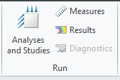
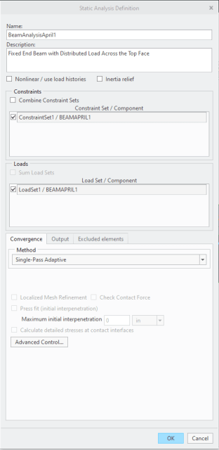
Creating and naming a study is mostly auto-populated using the last sets of constraints and loads as defaults. This is one of the places where adding information into the “Description” field will help with documentation. If someone returns to this study for reference in six months, information about what you studied and how you loaded it will help the next person.

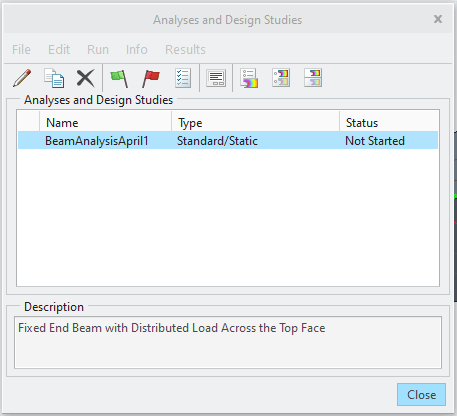
One of the lessons I like to teach is that documentation for the future person could also help you later, as you run hundreds of studies in a year, and the mind clouds from the multiple variations. The green flag lets you know that the study is ready to run. If any issues arise, several aggressive beeping windows will pop up with the error source.

Run the analysis. (Image: Tom Spendlove.)

The status window shows the run’s progress and statistics. (Image: Tom Spendlove.)

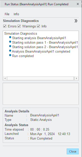
This was an extremely fast example, and the “Run Status” window shows that the entire study took 0.25 seconds. The window also shows that two adaptive passes were run — the system looks between each successive pass to see if multiple iterations deliver better results. It’s important to note that in most simulation studies, the setup and results communication require solid engineering and understanding, and the software needs enough computing power and graphics capability to plug and chug through the calculations.

After the simulation is run, select the “Results” tab. (Image: Tom Spendlove.)

The default “Results” window shows von Mises stress, displacement and principal stress vectors. (Image: Tom Spendlove.)

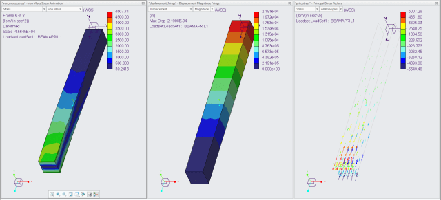
When I teach simulation using any software, I tell the students that the default Results window will generate a heatmap between cold blue and hot red. The software doesn’t necessarily know the material’s yield strength without indicating it beforehand, nor does it know what safety factor you want for this application. The software does what you tell it to do and then gives you the default displays. Presenting this information to a large group can be dangerous if you don’t explicitly set the context for the results.

Generally, it is most useful to find the areas of maximum stress and maximum deformation and then understand if those maximums work within the system you’re designing. Some applications might want to show vectors for stress or strain, and Creo has a wide array of displays for engineers to use.

The big thing to think about here is whether the results make sense. Should there be maximum stress on the attachment side and maximum displacement on the free-hanging side? That makes sense and aligns with what I would expect from this study. Just because we have powerful software that can do powerful things doesn’t mean we should unquestioningly trust any results that are spit out at the end of the process. Students often abandon the idea of even doing short back-of-the-envelope calculations once they’re comfortable running the software. However, you need a general idea of the expected results to maintain good engineering practices.

This basic beam deflection simulation shows the steps engineers can take to run a quick simulation, but it is only the tip of the iceberg of what Creo can do. The square beam section can easily be changed to an H- or I-beam configuration to be more realistic to construction standards. Square corners didn’t necessarily come into play here, but 90° angles are generally massive stress risers in simulation, and liberally applying fillets to all corners could save a lot of time troubleshooting results later. Instead of using the generic medium carbon steel material properties from the Granta functions of Creo, we could find the exact grade of steel used in our application and make those properties true to life.